Abstract

Smooth motion, meaning very low position and current loop error while at speed, is critical to system performance in many precision motion applications, including surgical and industrial robotics, optical scanning and inspection, and semiconductor equipment. Slotless motors provide smooth motion due to their inherent zero cogging design. These motors, however, have very low inductance due to their lack of iron in the magnetic field. Low inductance can create unwanted side-effects such as coil heating from PWM current ripple. This paper discusses how to configure a low inductance motor system to reduce current ripple and minimize position error while under motion. Configurations include PWM rate adjustment, adding inductors to each motor phase, and tuning the current loops. Some background regarding motors and driving inductive loads with a PWM drive will be discussed to set the stage for a thorough discussion of how to optimize a slotless motor system.

Slotless Motors vs. Slotted Motors

“Slotless” rotary motors do not have protruding poles (or salient iron teeth), making them physically look and perform differently than a typical “slotted” motor. Instead, slotless motor phase coils are typically form wound and inserted in the stack as opposed to being wound around the teeth of a slotted motor. (Refer to TN-2001 for a detailed explanation of slotted vs. slotless). Unlike a slotted motor where the rotor’s magnetic poles are attracted to the steel “teeth”, the lack of iron teeth in a slotless motor makes it have no naturally occurring torque cogging positions. The stable locations where a brushless dc (BLDC) motor’s rotor aligns with the stator teeth is called a “cogging” position. The servo system must push its way through these positions in order to rotate the motor. For this reason, slotless motors are the preferred choice when smooth motion is critical. There are no cogging forces that the servo must push through, which results in less position error while at speed.

For linear motors, the ironless linear motor is analogous to the rotary slotless and the linear iron-core motor is analogous to the slotted rotary.

Motor Poles

The number of magnet poles (and pole pairs) is a key characteristic of a brushless dc motor. The number of pole pairs (N/2), where N is the number of poles, defines the number of electrical cycles in one mechanical revolution. This is sometimes referred to as the “electromagnetic gear ratio”. When in motion, the electrical spatial frequency can be thought of in time as electrical cycles per second or Hertz (Hz). This frequency is a key parameter for which the current loop must be tuned appropriately.

Inductance

Any energized inductor has a voltage drop associated with the time-varying current through the inductor, (V = L * di/dt, where V is the voltage drop across the inductor, L is in the Henrys and di/dt is the time rate of change of current flowing in the circuit). Alternatively, one could state the time rate of change of current as a function of the voltage across the inductor and its inductance, (di/dt=V/L). We will use this formula later to calculate the current ripple created from the PWM drive.

The inductance of slotless motors tends to be much less than a slotted motor because the inductance is proportional to the permeance (ability to allow magnetic flux lines to pass) of the coil’s magnetic circuit. The presence of iron in the magnetic circuit, acting as a highly permeable path for the magnetic flux, makes the circuit permeance much higher. Therefore, slotted motors with iron teeth to conduct the magnetic flux have higher inductance than slotless motors.

PWM Drive Voltage and Inductive Loads

RL Load and Voltage PWM

Pulse Width Modulation (PWM) of the bus voltage to control the average voltage applied across the motor phases is a common way to drive motors. PWM motor drives are highly efficient and very cost effective versus linear drives. A PWM drive creates the desired dc current by varying the amount of on and off time (duty cycle) of the applied voltage. Using PWM to drive a motor, which has resistance and inductance, creates a dynamic current waveform based on the time constant of the RL circuit. Figure 1 below shows how current will rise and fall as the PWM voltage is applied across an RL circuit. In this case, the PWM is at 50% duty cycle, and the RL time constant is less than the half period of the PWM rate, so the current is reaching its maximum, and minimum, before the next voltage transition. The average current shown is about 4 amps with 7.5 amp peak to peak of ripple.

Applied PWM voltage

Figure 1. Applied PWM voltage and subsequent current in a motor

Duty Cycle and Average Current

In order to create more or less average current, the PWM duty cycle is altered. For instance, the maximum current would be available if the duty cycle were 99.9% and conversely, the minimal current available when the duty cycle is at 0.1%. Figures 2, 3 and 4 below represent 50, 1 and 99% duty cycles.

2.5% PWM duty cycle

Figure 2. 2.50% PWM duty cycle

The 50% duty cycle is the worst case for current ripple. The current flowing in the coil has an equal amount of time to build up and decay, making the peak to peak ripple the worst case. For low inductance motors, the peak to peak ripple can be a significant percentage of the average value. Figure 2 above for a 50% duty cycle, shows a 3 ohm, 0.1 mH motor, having 2.85 amps pk-pk and a 4 amp average.

The blue curve, representing a motor with a more typical inductance of 1mH, is showing a slow build up to a steady state current. This reaction is caused by the larger RL time constant of resistive and inductive load.

The 1% duty cycle is shown below. In this case, current ripple for low inductance motors is much lower than the 50% duty cycle case, but it is still a large percentage of the average. In the 1% PWM case shown in Figure 3, the 3 ohm, 0.1 mH motor has 0.12 amps pk-pk and an average of 0.1 amps.

1% PWM duty cycle

Figure 3. 1% PWM duty cycle

The final case (shown in Figure 4) is the 99% duty cycle. In this case, the peak to peak current ripple is the same as the 1% case, but versus its average, it is a much smaller percentage.

99% PWM duty cycle

Figure 4. 99% PWM duty cycle

PWM Rate and Current Ripple

Motor power dissipation (motor heating) is often a concern for precision mechanisms. Depending on the application, current ripple created from PWM drives and low inductance motors can be a major contributor to motor heating. In the 50% duty cycle case shown in Figure 2 above, the peak to peak ripple is almost as large as the average current. For a motor with 1 amp of average current, and 0.6 amps of peak to peak (proportionally similar to the case shown in Figure 2), the RMS of the total current is 1 + 1/sqrt(3)*0.3 = 1.17 amps. This is a 17% increase over the average current. In motor power dissipation, the current is squared, so 1.17 amps squared becomes 1.37 amps and power dissipation increases by 37%. Thermal resistance is the measure of temperature rise per watt, so a 37% increase in dissipated power will equate to a 37% increase in temperature of the motor coil.

A simple way to reduce the dissipated power is to increase the PWM rate. Not all drive manufacturers will suggest doing this, as it puts more thermal load on the drive devices, which has likely not been evaluated at the proposed PWM rate and motor load. It is always recommended discussing these issues with the drive company’s Applications Engineers and inform them of any motor power dissipation concerns when driving a low inductance motor.

The formula for voltage drop across an inductor (described earlier) can be used to calculate the maximum amount of current ripple in a motor. In this calculation, care must be taken in using the correct voltage. For example, when evaluating current ripple at very low speeds, we can typically ignore Vbemf.

When the back emf becomes larger than 10% of the bus voltage, it must be subtracted out to get an accurate current ripple calculation.

Current ripple calculation

Figure 4. 99% PWM duty cycle

Equation 1. Current Ripple from PWM Rate and Vbus

In this section, current ripple versus PWM rate is compared using a low inductance motor (0.1mH). Figure 5 below shows how doubling the PWM rate will half the peak to peak current ripple. The reduction in ripple is coming from the reduced time available for current to rise and fall based on the RL time constant.

Current ripple vs PWM rate

Figure 5. Current Ripple vs PWM for 1 amp command (Red – 20KHz, Blue – 40KHz)

15-20 KHz is a typical PWM rate found on most drives. 30-40KHz is available from several manufacturers but requires significant setup and discussion to implement and is often not clearly documented, 60-100KHz is available from a small number of suppliers and can dramatically reduce current ripple. Figure 6 is a compilation of locked rotor test data from three common drive manufacturers. A locked rotor test means that the rotor is not allowed to spin while a constant current is being commanded to the drive. A current probe was used across one of the motor phase leads. The rotor was rotated manually to find electrical angle such that the phase current for the probe was at its maximum. The data clearly shows three key points. Observation 1 is that higher PWM rates result in lower amounts of current ripple. Observation 2 shows how all three drive companies have similar performance. The third point, which is less obvious, is that one of the three drive companies did not offer an 80 KHz PWM rate. PWM rates is parameter that should be discussed with the targeted drive manufacturer when using slotless motors.

Current Ripple vs Drive Company vs Drive Level

Figure 6. Current Ripple vs Drive Company vs Drive Level

Add on Inductors

If a drive does not support medium to high PWM rates, meaning greater than the standard 15-20 KHz range, and current ripple (motor heating) is still a concern, adding inductors in series with each motor phase is an option. The added inductance does come with added resistance and a loss of efficiency, but it can significantly reduce current ripple and make the motor run cooler. Figure 7 below shows how doubling the inductance achieves the same ripple and doubling the PWM rate. When using add on inductors, care must be taken in correctly sizing the inductors by current capability or power dissipation. Generally, this is only a viable option with low current drives as inductor sizes can quickly exceed motor sizes as the required current levels increase. Other factors involved with add on inductors is that they require new current loop tuning, as the RL pole in the plant will have shifted, and require additional cabling for connecting to each motor phase. In many applications, this option is simply too complicated due to space limitations.

Current Ripple with Added Inductance

Figure 7. Current Ripple with Added Inductance

Control Architecture

Inner and Outer Loop Architecture

Rotary motion control is typically achieved through the use of at least two nest control loops, an inner current loop and outer position loop, (see Figure 8 below). A velocity loop is sometimes added between the slow position loop and fast current loop.

Nested motion system architecture

Figure 8. Nested motion system architecture

In the nested loop architecture, the current loop’s function is to deliver current based on the torque needed to make the outer position loop error a minimum. Typically the current loop bandwidth is ten to twenty times higher than the positon loop bandwidth, putting it near or greater than 1 KHz. Tuning of these two servo loops has a direct effect on how well slotless motors perform in any motion system.

Target Current Loop Bandwidth

Before any current tuning begins, the maximum operating speed and pole count must be used to calculate the electrical cycle frequency for the system. The formula is simply; N/2 * RPM/60, where N is the number of poles and the units are electrical cycles per second. The current loop gains must be tuned so that the bandwidth is at least 2 to 3 times greater than the electrical cycle frequency, allowing the drive to produce phase current instantly, as the commutation algorithm switches the applied current into the correct phases throughout a mechanical revolution.

Current Loop Tuning

Two phases of a BLDC motor can be represented as a simple RL circuit, which when represented in the LaPlace domain takes the form of a 1st order system Current loop tuning. It turns out, however, this RL, 1st order transfer function changes when we consider the effect of the motor’s back emf. If we simulate the effect

of back emf, the “Plant” for the current loop becomes the entire block diagram shown in Figure 9 below. As more back emf is allowed to flow, the transfer function changes from a first order shape, to a second order transfer function that transitions from +1 slope to -1 slope in magnitude and +90 to -90 degrees in phase (see Figure 10.). This dramatic change in the transfer function would normally be considered detrimental for a fixed PI control law. In this case, however, the change is towards stability, not away from it (meaning phase is added, not removed), making the loop stable when the motor is at rest, and while moving.

Motor transfer function

Figure 9. Block Diagram of the Motor Transfer Function

Motor Plant Transfer Function vs Back EMF Factor

Figure 10. Motor Plant Transfer Function vs. Back EMF Factor

Controlling the plant transfer function shown in Figure 10 requires only a Proportional + Integral (PI) controller with an additional first order low pass filter on the current sensor. The low pass filter is typically at a fixed value in the drive software, therefore the user doesn’t typically tune this value. Tuning the current loop is almost always done with a step response tool within the drive software. In some cases, a higher fidelity tuning method is needed to get the absolute maximum performance out of the current loop. In that case, tuning is suggested to be done in the frequency domain using Bode Plots. We will first discuss current loop tuning within the time domain, then move into some more advanced tuning in the frequency domain using Bode Plots.

Figure 11 below is simulated data from a low inductance slotless motor. The plot contains many curves, each with different PI gains. As the PI gains are increased, the response gets closer and closer to the commanded step in current. The green trace would be considered by most to be the best combination of response time and overshoot. In some applications, however, more performance is needed, and overshoot is a metric that can be relaxed at the benefit of better disturbance rejection. Having a small amount of overshoot, without subsequent oscillation is a stable gain set and is the highest gain possible for the system. Many drive manufacturers do not recommend this level of tuning, as in some cases it can interact with high frequency structural resonances and create an audible tone or worst case, an instability. Depending on the application, however, this level of tuning can give the system the extra performance it needs. In Section 5, optimal I gain tuning is discussed and it is shown how higher I gain values yield better disturbance rejection.

Position Loop Tuning

Position loop tuning is critical in determining how a precision mechanism or motor system moves and settles. Tuning the position loop, however, is not directly affected by the motors’ inductance. The “Plant” for the position loop is really the inner current loop plus the inertia of the motor shaft (or moving structure) and any structural dynamics it may have. The challenges of position loop tuning are related to these structural dynamics and any time lags between the motor and the sensor. These concepts are not discussed here, as this paper is focusing on tuning for low inductance motors.

Advanced Current Loop Tuning

In Section 4, time domain tuning of the current loop’s PI gains was discussed. In that section, it was shown how P and I gain affect the time response from a step input of current. In this section we will discuss how the P and I gains shape the loop transfer function in the frequency domain.

Frequency Domain Tuning

Position and integral control are represented in the LaPlace domain as GGGGRRCC ∗ bb+AAbb, where A = Ki/Kp and Gain = Kp. This form of PI control is important to note because it tells the control designer that at frequency “A” the integrator turns on (or off). Turning the integrator “on” at a higher frequency means that the gain will be higher for all frequencies below A (see Figure 13 below). The beauty of frequency domain tuning is that the control designer can visually see how the Ki gain only increases loop gain below the corner frequency A, and not above. When tuning in the time domain, this effect is not observable. Increasing only low-frequency gain is critical when the system has high-frequency resonances above frequency A that might have Gain Margin sensitivities.

In control design, we must often make decissions and tradeoffs based on the applications needs. In this case, the benefit we get from increasing low frequency gain causes lost phase near the targeted servo bandwidth. Turning the integrator on at a higher frequency means the amount of phase margin at the bandwidth is reduced. Figure 13 below shows how the phase from PI control changes with frequency and specifically, you can see that at the targeted bandwidth (the green circle), there is about 15 degrees of phase loss from the 10xKi case versus the Ki gain case.

I Gain effect on Bode Plot

Figure 11. I Gain Effect on Bode Plot

To complete this discussion of frequency domain tuning, we should discuss how Kp, gain affects the loop transfer function. Above we stated that a PI controller is represented as GGGGRRCC + bb+AAbb, where A=Ki/Kp and Gain = Kp. In Figure 14 you will notice that if we change Kp, we change both the integrator frequency A and the high frequency gain value. The combined effect of a change in “Gain” and the corner frequency A, essentially keeps low frequency gain unchanged, and increases high frequency gain. It also affects the phase curve in that more phase margin would be available since the corner frequency has been reduced.

Changing only Kp

Figure 12. Changing only Kp

Example Using High I Gain

In this section, we will discuss an example of how increased I gain compensation can be used to improve current loop performance. As mentioned earlier, an ironless linear motor is in many ways equivalent to a rotary slotless motor. Below is a simplified picture of the workings of a linear motor.

Linear Ironless Motor

Figure 13. Linear Ironless Motor

In this picture, forces are created from the interaction of the current running through motor phases A, B and C and the corresponding magnetic field due to the individual magnets. This interaction of current and magnetic field is captured in the motor parameter Kf (N/amp). Each individual magnet, however, has slightly different magnetic strength causing the magnetic fields to correspondingly vary in strength. This in turn causes the motor’s Kf to vary in strength as a function of position and ultimately causes the forces Fa1 through Fc2 to vary in strength with position. Other contributors to position dependent force variability are magnet spacing, motor coil to coil spacing, and motor coil turn spacing. All of these combine to create a varying Kf with position.

As mentioned earlier, the motor parameter that captures this conversion of applied current to force is the force constant of the motor (Kf). When using SI units, the back emf constant is numerically the same as the force constant. So, as the coil moves through the varying magnetic field, the back emf constant also fluctuates, thereby creating a fluctuating back emf voltage. The varying loss of voltage as a function of position is subtracted from the bus voltage, and the remainder is applied across the coil to make current. The block diagram below shows where the back emf loss is accounted for in relation to the current loop and a simplified RL motor model. The current loop’s job is to keep the desired current correct while any voltage disturbances are taking place. In this case, as the coil moves through the varying magnetic fields, there is a voltage disturbance (in the form of back emf) that the current loop must correct for. In the block diagram, this is captured through at the sum block just before the coil model.

Current loop and motor with varying Kf

Figure 14. Block diagram for current loop and motor with varying Kf (ke).

The frequency of the voltage disturbance is critical. For slow speeds, the frequency is also slow, as the frequency is the linear speed in mm/sec divided by the magnetic pitch (mm/pole pair or electrical cycle). The units here become electrical cycles per second or “Hz”. At the low speeds (and low frequencies), the loop gain is very high (see Figure 17). In these regions, it may be difficult to see any benefit of optimal integrator tuning because the gain is so high that improvement may be in the noise of the measurement. At higher speeds (and frequencies), however, maximizing I gain could lead to a two or three times improvement in current ripple from varying Kf.

RL Plant and Loop Transfer Function plot

Figure 15. RL Plant and Loop Transfer Function plot for low and high gain current loop

For this example, a 200 Hz sinusoidal signal was injected into the voltage summation block. The amplitude of the sinewave was set using a Ke value of 10 volts per m/sec, at a speed of 0.5 m/sec and a variation of 10% of that that value. What this means is that Kf (or Ke), will vary +/- 10% at a frequency of 200 Hz. This is used to represent how a linear coil moves through a motor track with varying magnets strength. The varying Ke will cause a fluctuation at 200 Hz of the back emf component of coil voltage. This fluctuation will act as a disturbance to the voltage being applied to the coil. Figure 17 shows the two Loop Transfer functions that were evaluated. Both have a 0 dB cross over frequency of approximately 2 KHz (bandwidth), but have different low frequency gains due to the different I gain used. At 200 Hz, the gain difference is about 10 dB, which is a factor of 3. The net benefit of the 3x in gain is shown in Figure 18 where the higher Ki case is clearly performing better by about 2 to 1. It should be noted that if the back emf voltage model were applied for this example, the red curve would be shaped like the red trace of Figure 10, but with a peak at 400 Hz, and the slope of the green and blue curves would flat below 400 Hz, separated in amplitude by the same amount as shown here.

Drive companies will typically not recommend this level of advanced tuning as it tends to reduce phase margin of the current loop. The amount of acceptable Phase Margin is not the same for every application. In mechanical systems, closing loops with 30 degree is margin is common practice, while in electrical engineering disciplines, like op-amp design, loops are closed with a minimum of 60 degrees margin. The I gain optimization described here can become a very useful tool for the right application. The higher level take away from this discussion, however, is that when tuning a control law to reject tonal frequencies, gain is what is important, not bandwidth. As shown above, two systems with the same bandwidth perform much differently against a tonal disturbance.

Current Loop Error vs I Gain

Figure 16. Current Loop Error vs. I Gain

Summary and Conclusions

Optimizing performance of a slotless motor driven by a PWM voltage drive requires knowledge of how a resistive and inductive load behaves under varying applied voltage. Understanding the tuning principals of the proportional and integral controlled current loops is also essential for getting the most out of the slotless motor system.

This paper discusses some basic motor and drive concepts including pole count, inductance, and PWM voltage. The difference between a slotless and slotted rotary motor was discussed and it was noted how slotless motors typically have low inductance. The fast RL time constant of a slotless motor, in combination with a PWM drive, creates current ripple that can be a significant contributor to dissipated power in a motor. Different approaches to reduce current ripple, including PWM rate, and added inductance were discussed. Increasing the PWM rate or adding inductance were both shown to be highly effective in reducing current ripple. Three common PWM drive manufacturers were tested and compared for current ripple and all were found to be similar in their performance, but not all offered an 80 KHz PWM rate.

Time domain current loop tuning was discussed and it was shown how current loop proportional and integral gains affect rise time and overshoot. Advanced frequency domain tuning was discussed where it was shown how P and I gain shape the gain and phase vs. frequency curves. The take away from frequency domain tuning is that changing I gain alters only the low frequency part of the gain curve, so as to not adversely affect any resonances in the system at higher frequency. This benefit of increased low frequency gain is at the expense of lost phase at the targeted bandwidth, so care must be taken to not destabilize the loop when optimizing I gain.

The concept of maximizing I gain was taken to a simple motor example, where a voltage disturbance was an input to the commanded voltage across a resistive and inductive load (i.e. a motor). It was shown that the current error was reduced by a factor of 2 with optimizing I gain tuning.

PWM rate, additive inductance, and current loop tuning are all “tools” one can use to optimize performance of slotless motors with PWM drives. Using these techniques will enhance the inherent smooth motion benefit of a slotless motor.