


")

Position sensors are used in a wide range of automation and measurement applications. A key step in selecting a suitable position sensor is understanding the requirements of sensor size, resolution, repeatability, accuracy, mounting constraints and environmental ruggedness. This paper discusses the available position sensing technologies and concludes with a key feature comparison.
Position Sensors – Key Terms
Incremental Sensor
Provides position change information only so the actual position is unknown at startup. A once-per-rev index/marker signal defines the zero position or null of the device. It is detected during a homing routine. For commutation of a brushless motor the motor typically has three magnetic Hall sensors to provide coarse absolute position information for preliminary alignment of the magnetic fields. Incremental sensors are typically small, accurate and cost-effective.
Provides the actual physical position within one revolution or within the range of linear travel. The motor does not require Halls and homing is only necessary for rotary applications if the range of movement exceeds one revolution. The sensors are usually bigger and more expensive than incremental devices.
Multi-Turn
Rotary devices, the sensor provides actual position over multiple revolutions. Homing can be completely eliminated. Multi-turn devices incorporate internal gearing and are the most bulky, expensive solution.
Resolution
Defines the smallest position increment that can be moved or measured and is typically expressed in “counts”. High resolution is required for high performance servo systems. A positioning system “dithers” between two counts so the higher the resolution the smaller the dither. Resolution also has a significant impact on velocity ripple at low speed. Since velocity is derived from position feedback, if the resolution is low there may be insufficient data in a sample to accurately derive velocity. At high speeds, high resolution devices can generate data rates beyond the tracking capability of the controller or servo drive.
Interpolation
As will be seen, many sensors generate sine and cosine signals. The period of these signals is defined by the inherent “pitch” of the device. With sin/cos information it is theoretically possible to have infinite resolution by computing the ratio of the signals. This technique is known as interpolation. In practice, the fidelity of the sin/cos signals and signal to noise ratio limit the realizable resolution.
Accuracy
Defines how close each measured position is to the actual physical position. Accuracy is very much a system issue and can be dominated by mechanical errors such as eccentricity, straightness and flatness. Sensor errors include non-accumulating random variations in pitch (linearity), accumulating pitch errors (slope) and variations in fidelity of internal sin/cos signals. Precision machine builders typically calibrate out errors via a lookup table of offsets. More detail can be found in our Technical Paper ‘Understanding Resolution, Accuracy, and Repeatability’.
Repeatability
Defines the range of measured positions when the system is returned to the same physical position multiple times. Repeatability can be more important than absolute accuracy. For system inaccuracies to be effectively calibrated it is important for each position reading to be consistent. Sensor hysteresis (different readings depending on direction of approach to measure position) is an important factor in repeatability.
Modular
The most common form of rotary feedback device is packaged in an enclosure with internal bearings and a shaft for connection to a motor via a flexible coupling. The enclosures are available with a range of sealing ratings and are bulky. Modular devices have no enclosure or bearings and must be built into the mechanical system. They are significantly more compact but may require a more benign environment depending on the technology.
On/Off Axis
For rotary applications the sensor is typically positioned off-axis on the circumference of a scale which wraps around the axis of rotation. Some implementations position the sensor on-axis minimizing size when radial space is constrained.
Potentiometers
Although there is a trend towards non-contact sensors, potentiometers (‘pots’) are still widely used in lower-end applications. Pots measure a voltage drop as a contact(s) slides along a resistive track. They are available in rotary, linear or curvilinear forms and are generally compact and lightweight. A simple device will cost pennies, whereas a higher precision version may cost upwards of $200. Linearity of less than 0.01 per cent is possible by laser trimming the resistive tracks.
Potentiometers are best applied in lower performance applications with low duty cycles in benign environments. They are susceptible to wear and foreign particles such as dust or sand. Pots theoretically have infinite resolution but in practice resolution is limited to the analog to digital converter (ADC) interface and the overall noise environment.
Potentiometers Strengths & Weaknesses
| Strengths | Low cost; simple; compact; lightweight. Can be made accurate |
| Weaknesses | Wear; vibration; contamination, extreme temperatures. |
Optical Encoders – Transmissive

The transmissive encoder uses optical scanning of a fine grating or “scale” illuminated by an LED light source. The scale, rotary or linear, is made of transparent and opaque “lines” that are arranged in a 50-50 duty cycle. The number of transparent regions on the disc corresponds to the scale pitch which defines the resolution of the encoder.
The sensor generates a voltage in proportion to the incident light intensity. As the sensor moves relative to the scale the voltage varies sinusoidally. A second light detector is added 90° out of phase. This relates to a displacement of half a scale line. Whether the signal from sensor A leads sensor B or vice versa defines the direction of relative motion. The encoder output can be sin/cos signals but the signals are more typically converted to square waves: A quad B (quad relates to 90° phase shift). A controller detects transitions on the edge of each square wave which effectively increases the encoder resolution by a factor of 4.
The detectors tend to be large compared to the width of each line. At higher resolutions this can lead to spillover between channels. Adding a mask that matches the pattern of the channels helps clean up the signal. The trade-off with this type of design is that the air gap between scale and sensor must be very small imposing strict specifications on disc parameters such as flatness, eccentricity, and alignment making the device more vulnerable to shock and vibration.
Phased-array incremental encoders use solid state technology to provide a more robust solution. Instead of a discrete detector for each channel, a phased-array encoder features an array of detectors so that each channel is covered by multiple detectors. This approach averages the optical signal, minimizing variations introduced by manufacturing errors like disc eccentricity and misalignment, improving performance while relaxing fabrication tolerances.
Inherently incremental, the encoder typically has an additional scale track with a single transparent line and separate sensor. The sensor generates an index signal defining the null position of the device. Absolute versions of transmissive encoders incorporate multiple tracks, light sources and sensors which completely define position within a revolution. With mechanical gearing of one disc to second disc it is possible to define position over multiple revolutions.
Transmissive Optical Encoder Strengths & Weaknesses
| Strengths | Moderate resolution; good accuracy; high repeatability; cost-effective. |
| Weaknesses | Bulky; environmental ruggedness for modular devices. |
Optical Encoders – Reflective

The principle of the reflective optical encoder is very similar to the transmissive encoder. A reflective encoder works by emitting light from the same side as the sensor (relative to the code disc), and selectively reflecting portions of the light to the sensor. Reduced physical dimensions is a clear advantage of this solution. Without the collimation optics typically required in a transmissive encoder, and with the LED light source on the same side as the sensor, the total volume of the encoder can be reduced substantially. Resolution and accuracy is typically not as good as the transmissive encoder.
Reflective Optical Encoder Strengths & Weaknesses
| Strengths | Moderate resolution and accuracy, high repeatability; cost-effective |
| Weaknesses | Environmental ruggedness |
Optical Encoders – Interferential

A coherent laser light source generates a diverging beam which illuminates a diffraction grating pattern printed on the scale. The grating pattern is created using either chrome deposition on a glass scale or laser written lines on a metal tape scale. The 20µm pitch grating diffracts the light to generate a high contrast interference pattern of bright and dark directly back onto a detector array. Inherently incremental, a second index/marker track is typically provided.
The diffracted light creates discrete Talbot planes of interference patterns. In the example above the 3rd Talbot plane is utilized. As the relative position of the scale and detector changes, the diffraction pattern translates across the detector array resulting in a sinusoidal change in each detector cell.
Interferential technology requires minimal optical components resulting in a sensor of small size. Resolution, without interpolation, is typically more than order of magnitude higher than transmissive or reflective optical encoders. Because of the fidelity of the sine and cosines signals high interpolation is possible yielding nanometer resolution with high accuracy. Considering the precision of the device, alignment tolerances are not excessively demanding.
This type of encoder requires a clean environment. Employing a less coherent LED light source combined with collimating and filtering optics significantly improves contamination immunity. The encoder is inevitably larger and typically has tighter alignment tolerances. See TN-1001 and TN-1002 for more details.
Interferential Optical Encoder Strengths & Weaknesses
| Strengths | High resolution, accuracy, repeatability; compact; moderate alignment tolerances |
| Weaknesses | Environmental ruggedness for Talbot plane implementation. |
Absolute Techniques for Optical Encoders

The absolute scale shown above has multiple codes similar to bar-codes. The number of code bits determines the number of unique codes and hence the maximum length or circumference of the scale. A camera captures the code and subsequent processing determines absolute position. There is an increased latency (time to get a reading) in this technique. Some encoders revert to an incremental track after the initial absolute reading to reduce latency. The interface to this type of encoder is typically a serial interface such as BiSS-C or SSI (see TN-1057).
The bar-code technique can be expensive. A much more cost-effective solution employs what are essentially multiple indexes. Each pair of indexes is separated by a unique number of lines as seen on the incremental track. At startup it is necessary to cause motion so that two indexes are detected. During this process the number of lines on the incremental track are counted. Using a lookup table the absolute position can determined. The downside is the requirement for movement before absolute position is determined.
Absolute Optical Encoder Strengths & Weaknesses
| Strengths | Good resolution, accuracy, repeatability; moderate alignment tolerances |
| Weaknesses | Environmental ruggedness; can be expensive for true absolute. |
Magnetic Encoders

A magnetic encoder employs a multi-pole magnet track. The sensor, Hall-effect or magnetoresistive, measures the change in magnet flux as the magnetic poles move relative to sensor. Sine and cosine signals can be generated as in the optical encoder.
A magnetoresistive resistor is formed from a magnetically sensitive alloy such as nickel iron. An external magnetic field stresses the magnetic domains of the material, changing the resistance. A magnetoresistive sensor consists of an array of lithographically patterned thin-film resistors. As the rotor poles pass by the sensor array the resistance changes sinusoidally.
A Hall sensor consists of a layer of semiconductor material, typically p-type, connected to a power supply. An applied magnetic field exerts a force (Lorentz force) on the charge carriers, causing them to separate to create a potential difference. The Hall sensor generates a voltage which is dependent on the strength of the perpendicular component of the magnetic field.
The device is inherently incremental and the illustration above shows an index track to define the null position. A second sensor and magnetic track with a different pole count can be added. A combination of the readings from each track is used to determine absolute position.
Magnetic encoders are rugged, compact and can be very cost-effective. They are, however, susceptible to magnetic fields and crosstalk can occur between sensors in close proximity. It is difficult to produce a fine pitch magnetic track limiting resolution. Repeatability is compromised by hysteresis and accuracy changes over operating temperature range. The magnetic track is relatively brittle and can be susceptible to shock.
Magnetic Encoder Strengths & Weaknesses
| Strengths | Robust; compact; tolerate liquids and non-metallic contaminants; on-axis versions |
| Weaknesses | Temperature; hysteresis; susceptible to magnetic fields; impact/shock resistance. |
Capacitive Encoders


Capacitive encoders are based on the principle that capacitance is proportional to the dialectric material between two charged plates. As shown in the illustration, an electric field is created between the capacitively coupled transmitter and receiver. The rotor sinusoidally modulates the dielectric ԑ causing a change in capacitance. The change in capacitance in turn modulates the potential difference between transmitter and receiver. Multiple modulating tracks are employed to define absolute position.
Capacitive encoders are compact and consume very little power. They are, however, susceptible to condensation and electrostatic build-up. Capacitance also varies with temperature, humidity, surrounding materials and foreign matter, which makes engineering a stable, high accuracy position sensor challenging. The components of the device have very small air gaps requiring careful installation.
Capacitive Encoder Strengths & Weaknesses
| Strengths | Compact; low power. |
| Weaknesses | Environmental ruggedness; alignment tolerances. |
Resolvers


Resolvers are based on the principle of electromagnetic induction – an alternating current in one conductor generates a changing magnetic field around the conductor. This magnetic field can induce an alternating current in an adjacent conductor. The magnitude of coupling from one conductor to another depends on the rate of change of magnetic field and the relative position and geometry of the conductors.
As shown below, a 5kHz (typ.) sinusoidal reference voltage in the stator induces a sinusoidal voltage in the rotor winding. A second, axial, rotor winding then induces a voltage in two axial signal windings displaced by 90º back on the stator. The amount of coupling into the stator windings is a function of the relative position of the rotor which effectively amplitude modulates the stator signals as shown.
In the illustration above the rotor is shown outside the stator for clarity. The radial windings on the stator interact with only the radial windings on the rotor. In turn, the axial windings on the rotor interact with only the axial windings on the stator. This is to avoid the stator reference winding coupling to the stator signal windings. Winding a resolver is not trivial and the end result is a heavy, bulky device. The resolver does, however, have unmatched ruggedness as there are no electronics or fragile parts in the device.
Resolvers are available in various “speeds”. A single speed resolver has one electrical sinewave cycle per rev and provides absolute position information with limited resolution. A “multi-speed resolver” is wound for a higher number of electrical cycles per rev improving resolution. The higher ratio of electrical to mechanical cycles also helps minimize the effects of mechanical error sources. Multi-speed resolvers are no longer absolute and are more expensive and typically even more bulky.
Resolver Strengths & Weaknesses
| Strengths | Moderate resolution and accuracy; reliable; extremely robust |
| Weaknesses | Expensive; bulky; heavy. |
Inductive Encoders

The absolute inductive encoder is based on the same electromagnetic induction principle as the resolver but uses PCB traces rather than coil windings. The TX track on the stator is excited by specific frequency in the range 1-10MHz. This signal inductively couples into target with a resonant LC circuit. The target magnetic field induces a sinusoidal current in stator RX track. The RX track is sinusoidal in shape which effectively amplitude modulates the induced signal. A second RX track displaced by 90º carries a cosine signal. The sin/cos signals are interpolated and output as BiSS-C, SSI or in some versions AqB signals.
The RX tracks on the stator are analogous to a twisted pair wire. The balanced dipole effect cancels electric fields induced in the RX tracks from the changing magnetic field on the TX track. The RX track responds to changing magnetic field on the target only. The RX tracks also reject external electromagnetic interference. Undesirable induced stator currents are also rejected based on frequency and phase.
The main RX tracks with one sin/cos cycle per rev defines absolute position. A secondary track with multiple cycles enhances resolution. More typically the main TX track has multiple cycles (9 for example) combined with a secondary track with a number of cycles not a multiple of 3 – every position within one rev is defined by two unique readings.
The use of PCB traces versus the resolver’s windings brings significant advantages including: reduced cost, size and weight; form factor flexibility including curvilinear; elimination of inaccuracies from the winding process; for safety-related applications multiple sensors can be located in the same space by using multi-layer circuit boards.
The PCB material is environmentally very stable. The option for remote electronics further increases ruggedness. The 360º sensor improves eccentricity error tolerance.
Inductive Encoder Strengths & Weaknesses
| Strengths | Moderate accuracy and resolution; reliable; robust; multiple geometries; compact; lightweight |
| Weaknesses | Typical minimum diameter is 37 mm. |
Position Sensors – Technology Comparison
A comparison of position sensor / position feedback devices is shown below. Reflective encoders can be considered similar to transmissive encoders. Potentiometers are excluded as they are contact devices.

Technology comparison of position sensors
The ultimate goal is to find the most cost-effective solution that meets the requirements of precision, size and ruggedness. Two things stand out from the chart above: the interferential encoder is the clear leader in terms of precision and size; resolvers and inductive encoders lead with a combination of environmental ruggedness and moderate precision. As discussed, the inductive encoder has numerous advantages versus the resolver particularly size and weight.